Here we’ll look at how latent-variable models can be manipulated to yield an unbiased estimator of the marginal log-likelihood. We’ll implement the recently proposed SUMO (Stochastically Unbiased Marginalization Objective) in Jax, highlighting how Jax differs from standard Autodiff frameworks in some major aspects. Section 1 concerns the derivation of the SUMO objective. Section 2 walks through the Jax implementation, while section 3 contains the obligatory toy problem. This post did turn out longer than expected, so you may want to take a breather between sections. If you are only interested in the practical part, skip to Section 2 or check out the associated repository on Github.

• 1. SUMO
  • 1.1. Russian Roulette
  • 1.2. Estimator
  • 1.3. Variance Reduction
• 2. Implementation in Jax
  • 2.1. Defining the IW-ELBO
  • 2.2. Defining the SUMO estimator
    • 2.2.1. jit Technicalities
• 3. Density Matching
  • 3.1. Objective Function
  • 3.2. Optimization
  • 3.3. Contour Density Plots
• Conclusion
  • Credits
  • References

1. SUMO

The SUMO (Luo et. al., 2020, [1]) estimator makes use of the importance-weighted ELBO (IW-ELBO), examined in an earlier post. Briefly, we are interested in finding a lower bound of the log-marginal likelihood $\log p(x)$. Under certain conditions, the tightness of this bound scales with the variance of some unbiased estimator $R$ of the marginal probability. $R$ depends on the latent variables through some proposal distribution $q(z)$: $\E{q}{R} = p(x)$. The regular VAE takes $R = p(x,z)/q(z)$, forming the normal ELBO $\E{q}{\log p(x,z) - q(z)}$, but a natural way to reduce the sample variance is through the $K$-sample mean, forming the IW-ELBO:

Here to be consistent with the notation in [1], we define this without the expectation under $q$. One can show [2] that the IW-ELBO is monotonically increasing in expectation and converges to the true log-marginal likelihood as the variance vanishes as $K \rightarrow \infty$:

So it appears we can only obtain an unbiased estimator of $\log p(x)$ after doing an infinite amount of computation.

1.1. Russian Roulette

SUMO circumvents this difficulty by randomized truncation of a specially constructed infinite series - falling under the class of the so-called ‘Russian roulette estimators’ [3]. Where exactly the specific form of the estimator comes from in the paper is a bit mysterious, so we’ll motivate it heuristically below. For a general discussion, let $\Delta_k$ be the $k$th term of some series that converges to some quantity of interest $p^* = \lim_{K \rightarrow \infty} \left( \sum_{k=1}^K \Delta_k\right)$. We want to truncate the series at some finite stopping time $K$, while retaining unbiasedness.

This is possible if we treat $K$ as a discrete random variable with mass function $p(K)$ with support over the natural numbers. The core idea is to draw $K \sim p(K)$, evaluate the first $K$ terms in the sum (each appropriately weighted to account for truncation), and stop. Taking the expectation of the partial sum w.r.t. $p(K)$ and shuffling things around in the resulting double sum¹:

Where $\mathbb{P}(K \geq k)$ is the complement of the CDF. This suggests we can obtain an unbiased estimator of the infinite series by first sampling the stopping time $K$, and then evaluating $K$ appropriately weighted terms²:

1.2. Estimator

To connect this back to lower bounds on $\log p(x)$, note that the following telescoping series converges to $\log p(x)$ in expectation in the limit:

Let $\hat{\Delta}_k(x)= \E{q}{\textrm{IW-ELBO}_{k+1}(x)} - \E{q}{\textrm{IW-ELBO}_k(x)}$ then apply the Russian roulette estimator to the sequence of partial sums:

Luo et. al. [1] define the interior of the expectation to be the Stochastically Unbiased Marginalization Objective (SUMO) estimator, which is equal to the marginal log-probability in expectation over $K$ and $q(z)$:

Defining $\Delta_k(x)= \textrm{IW-ELBO}_{k+1}(x) - \textrm{IW-ELBO}_k(x)$, we arrive at the slightly more palatable form:

1.3. Variance Reduction

As Lyne et. al. [3] (Appendix A.2.) demonstrate, the variance of the generic Russian roulette estimator can be potentially infinite - there is a tradeoff between computation time (controlled by the expected value of the stopping time and hence the form of the PMF $p(K)$), and the variance of the resulting estimator. Luo et. al. [1] propose that the variance of SUMO can be minimized through optimization of the parameters $\phi$ of an amortized encoder $q_{\phi}(z \vert x)$, noting that:

Where $\nabla_{\phi}\left(\E{q_{\phi}, \, p(K)}{\textrm{SUMO}(x)}\right)^2= \nabla_{\phi} \left(\log p(x)\right)^2 = 0$ by virtue of SUMO being an unbiased estimator of $\log p(x)$, and we apply reparameterization w.r.t. $z$ in the last line to pull the gradient into the expectation. So here the latent variables are doing double duty - used to obtain a sequence of lower bounds on $\log p(x)$, and to minimize the variance of the resulting estimator.

2. Implementation in Jax

Jax is a machine learning framework described as the spiritual successor of autograd. Here’s the elevator pitch: numpy + automatic differentiation, plus:

• Any-order gradients of your functions w.r.t. any input parameters through jax.grad.
• Automatic vectorization of single-example code into batches throguh jax.vmap.
• Automatic parallelization of code across multiple devices through jax.pmap.
• Automatic generation of optimized computation kernels through jax.jit.

All the above primitives can be arbitrarily composed as well. From my experience, Jax was easy to come to grips with, sharing much of its minimalist interface with numpy/scipy. Furthermore, it’s blazingly fast out-of-the-box - switching from CPU to GPU/TPU requires almost no work, and it is straightforward to fuse your code into performant kernels or parallelize across multiple devices.

However, Jax adopts a functional programming, as opposed to an object-oriented model, in order for function transformations to work nicely. This imposes certain constraints that may be unnatural to users accustomed to machine learning frameworks written in Python (Torch/Tensorflow). Python functions subject to transformation/compilation in Jax must be functionally pure: all the input data is passed through the function parameters, and all the results are output through the returned function values - there should be no dependence on global state or additional ‘side-effects’ beyond the return values. This can be somewhat vexing to those of us accustomed to calling loss.backward() in Torch - in fact, there’s a very long list of common gotchas in Jax associated with this functionally pure constraint, but we’ll see that this is not too big a barrier once you get used to it.

This section is quite long, but implementing and optimizing the SUMO estimator will force us to deal with a surprisingly large cross-section of Jax, together with a large volume of gotchas (at the time of writing this, as of v0.1.69).

2.1. Defining the IW-ELBO

First we need a way to get the importance-weighted ELBO terms that appear in the Russian roulette estimator. This part is a modified version of the full discussion in an earlier post about the importance-weighted ELBO. We’ll start off with the most numpy/torch-like part of the code, defining convenience functions to evaluate the log-density of a diagonal-covariance Gaussian and to sample from a diagonal Gaussian using reparameterization.

import jax as jnp
from jax import jit, vmap, random
from jax.scipy.special import logsumexp

def diag_gaussian_logpdf(x, mean=None, logvar=None):
    # Log of PDF for diagonal Gaussian for a single point
    D = x.shape[0]
    if (mean == None) and (logvar == None):
        # Standard Gaussian
        mean, logvar = jnp.zeros_like(x), jnp.zeros_like(x)
    jnp.sum(-0.5 * (jnp.log(2*jnp.pi) + logvar + (x-mean)**2 * jnp.exp(-logvar)))
    
 def diag_gaussian_sample(rng, mean, logvar):
    # Sample single point from a diagonal multivariate distribution
    return mean + jnp.exp(0.5 * logvar) * random.normal(rng, mean.shape)

Note in Jax we explicitly pass a PRNG state, represented above by rng into any function where randomness is required, such as when sampling $\mathcal{N}(0,\mathbb{I})$ for reparameterization. The short reason for this is because standard PRNG silently updates the state used to generate pseudo-randomness, resulting in a hidden ‘side effect’ that is problematic for Jax’s transformation and compilation functions, which only work on Python functions which are functionally pure. Instead Jax explicitly passes the PRNG state as an argument and splits the state as required whenever we require more instances of PRNG. Check out the documentation for more details.

Here we are performing amortized inference - instead of learning variational parameters per-datapoint, we train separate neural networks to output the parameters of the approximate posterior $q(z \vert x)$ and conditional model $p(x \vert z)$. These are called the encoder/decoder, respectively. The variational parameters are then the collective parameters of these networks - shared between all datapoints. Using a standard Gaussian for the prior $p(z)$ and diagonal-covariance Gaussian distribution for the conditional and approximate posterior, the necessary samples to compute the IW-ELBO are obtained through reparameterization - see Section 3.2. of this earlier post for more details.

Due to the functional programming paradigm, defining the encoder/decoder networks in Jax is slightly different from Torch/Tensorflow, etc. The core idea is that the constructor for each layer in the network expects an argument specifying the output dimension and returns:

• An init_fun, which initializes the layer parameters.
• An apply_fun, which defines the forward pass of the layer.

The Jax-native stax library provides a straightforward way to compose layers into a single model, wrapping them together according to a user-defined structure, and returning an init_fun which initializes parameters for all layers in the model and an apply_fun which defines the forward pass of the model as the composition of the forward computations for each layer. See the documentation for more details. Here both the amortized encoder/decoder are defined as single-hidden-layer networks, where the output of each is split into two pieces - the mean and logarithm of the diagonal of the covariance matrix over the respective space. We’ll refer to the latter as the log-variance.

from jax.experimental import stax
def encoder_constructor(hidden_dim, z_dim, activation='Tanh'):
    activation = getattr(stax, activation)
    encoder_init, encoder_forward = stax.serial(
        stax.Dense(hidden_dim), activation,
        stax.FanOut(2),
        stax.parallel(stax.Dense(z_dim), stax.Dense(z_dim)),
    )
    return encoder_init, encoder_forward

def decoder_constructor(hidden_dim, x_dim=2, activation='Tanh'):
    activation = getattr(stax, activation)
    decoder_init, decoder_forward = stax.serial(
        stax.Dense(hidden_dim), activation,
        stax.FanOut(2),
        stax.parallel(stax.Dense(x_dim), stax.Dense(x_dim)),
    )
    return decoder_init, decoder_forward

encoder_init, encoder_forward = encoder_constructor(hidden_dim=hidden_dim, z_dim=z_dim)
decoder_init, decoder_forward = decoder_constructor(hidden_dim=hidden_dim, x_dim=x_dim)

The initialization functions accept:

• A PRNG state for random initialization of parameters
• A tuple specifying the dimensions of the network input.

They return:

• output_shape: A tuple specifying the dimensions of the network output.
• init_params: A tuple holding the initial network parameters.

rng = random.PRNGKey(42)
rng, dec_init_rng, enc_init_rng = random.split(rng, 3)
z_output_shape, init_encoder_params = encoder_init(enc_init_rng, (-1, feature_dim))
x_output_shape, init_decoder_params = decoder_init(dec_init_rng, (-1, latent_dim))

Next we define the log of the summand of the IW-ELBO estimator - i.e. $\log \frac{p(x, z_k)}{q(z_k \vert x)}, z_k \sim q$:

def iw_estimator(x, rng, encoder, enc_params, decoder, dec_params):
    """
    Single-sample estimator of the ELBO
    """
    # Sample from q(z|x) by passing data through encoder and reparameterizing
    z_mean, z_logvar = encoder(enc_params, x)  # Encoder fwd pass
    qzCx_stats = (z_mean, z_logvar)
    z_sample = diag_gaussian_sample(rng, *qzCx_stats)
    # Sample from p(x|z) by sampling from q(z|x), passing through decoder
    x_mean, x_logvar = decoder(dec_params, z_sample)  # Decoder fwd pass
    pxCz_stats = (x_mean, x_logvar)
    
    log_pxCz = diag_gaussian_logpdf(x, *pxCz_stats)
    log_qz = diag_gaussian_logpdf(z_sample, *qzCx_stats)
    log_pz = diag_gaussian_logpdf(z_sample)
    
    iw_log_summand = log_pxCz + log_pz - log_qz
    
    return iw_log_summand

Note when applying the forward pass through the encoder and decoder, we have to explicitly pass the parameters of each network as arguments - this is in line with Jax’s functional programming interface - functions should only rely on their arguments, not global state. If you don’t like this functional interface, the good news is that there are two projects - flax and trax which provide a more object-oriented interface for network construction (these are a lot more readable/hackable, IMO).

The manner in which we collect the summands for different samples $z_k \sim q(z \vert x)$ represents another significant point of departure from other autodiff frameworks. We have to arrange the summands into the estimator:

def iwelbo_amortized(x, rng, enc_params, dec_params, num_samples=32, *args, **kwargs):

    rngs = random.split(rng, num_samples)
    vec_iw_estimator = vmap(iw_estimator, in_axes=(None, 0, None, None))
    iw_log_summand = vec_iw_estimator(x, rngs, enc_params, dec_params)

    K = num_samples
    iwelbo_K = logsumexp(iw_log_summand) - jnp.log(K)
    return iwelbo_K

First, we split the rng states into num_samples new states, one for each importance sample. Next we make use of jax.vmap - one of the ‘killer features’ of Jax. This function vectorizes a function over a given axis of the input, so the function is evaluated in parallel across the given axis. A trivial example of this would be representing a matrix-vector operation as a vectorized form of dot products between each row of the matrix and the given vector, but vmap allows us to (in most cases) vectorize more complicated functions where it is not obvious how to manually ‘batch’ the computation. For brevity, you can read more about vmap via the documentation or this previous post.

The return result of vmap is the vectorized version of iw_estimator, which we call to get a vector, iw_log_summand, representing the log-summands $\log p(x \vert z_k) + \log p(z_k) - \log q(z_k \vert x)$ for each importance sample $z_k$. This will be a one-dimensional array with number of elements given by the number of importance samples $K$. Finally for numerical stability we take the $\text{logsumexp}$ of the log-summands and average this to give the final IW-ELBO(K). Note that parallelization was near-automatic here for the computation of the different importance sample summands using vmap - we didn’t have to keep track of a cumbersome batch dimension anywhere.

2.2. Defining the SUMO estimator

The SUMO estimator is pleasingly simple to implement, here are the basic steps:

1. Sample stopping time $K \sim p(\mathcal{K})$. In practice to lower variance the authors choose to compute at least $m$ terms, so the total number of terms evaluated in the partial sum is $K+m$.
2. Sample $z_k\sim q(z \vert x)$ for $k=1,\ldots, K+m$.
3. Compute log-summands $\log w_k = \log p(x \vert z_k) + \log p(z_k) - \log q(z_k \vert x)$ for $k=1,\ldots, K+m$.
4. Compute $\textrm{IW-ELBO}(k) = \texttt{logcumsumexp}\left(\log w_k\right) - \log(k)$.
5. Return: $\textrm{IW-ELBO}(m) + \sum_{k=m}^{K+m} \Delta_k(x) \, / \, \mathbb{P}(\mathcal{K} \geq k)$.

We already did steps 2 and 3 above, let’s focus on step 1 - the authors propose the following tail distribution for the number of terms $\mathcal{K}$ to evaluate in the series: $\mathbb{P}(\mathcal{K} \geq k) = \frac{1}{k}$. This has CDF $F_{\mathcal{K}}(k) = \mathbb{P}(\mathcal{K} \leq k) = 1 - \frac{1}{k+1}$ and so by the inverse CDF transform $\left \lfloor{\frac{u}{1-u}}\right \rfloor \sim p(\mathcal{K})$, where $u \sim \text{Uniform}[0,1]$³. To reduce the possibility of sampling large stopping times, they flatten the tails of the CDF by heavily penalizing the probability of $k > 80$:

def reverse_cdf(k, alpha=80, b=0.1):
    return torch.where(k < alpha, 1./k, 1./alpha * (1-b)**(k-alpha))

We can tie this all together in the following function:

@partial(jit, static_argnums=(4, 5,))
def SUMO(x, rng, enc_params, dec_params, K, m=16, *args, **kwargs):

    rngs = random.split(rng, K+m)

    # Step 2, 3
    vec_iw_estimator = vmap(iw_estimator, in_axes=(None, 0, None, None))
    log_iw = vec_iw_estimator(x, rngs, enc_params, dec_params)

    # Step 4
    K_range = lax.iota(dtype=jnp.int32, size=K+m)+1
    iwelbo_K = logcumsumexp(log_iw) - jnp.log(K_range)

    # Step 5
    vec_reverse_cdf = vmap(reverse_cdf, in_axes=(0,))
    inv_weights = jnp.divide(1., vec_reverse_cdf(K_range[m:]))
    return iwelbo_K[m-1] + jnp.sum(inv_weights * (iwelbo_K[m:] - iwelbo_K[m-1:-1]))

2.2.1. jit Technicalities

What’s this business with the decorator? When Jax analyzes a function to compile using jax.jit, it passes an abstract value in lieu of an actual array for each argument, called a tracer value. These arrays are used to characterize what the function does on abstract Python objects - in most cases an array of floats - in order to be compiled using XLA. Tracer values share some functionality with ndarray - you can call .shape on these, for example - but forcing these to commit to specific numerical values will throw an error. Their only purpose is to characterize the behaviour of the function on a restricted set of possible inputs in order to be jit-compiled.

Tracer values are passed for each argument to the jit-transformed function, with the exception of those arguments identified as static_argnums by jit. These will remain regular values and treated as constant during compilation - with the caveat that when these arguments change, the function must be jit-compiled again. Hence, as the name suggests, static_argnums should not change too much to avoid incurring overhead from repeated compilation. Functions such as random.split and lax.iota do not accept tracer values as arguments, so we are forced to keep the sampled stopping time $K$ and minimum number of terms $m$ as regular Python values. This means, unfortunately, that each batch is restricted to use the same value of $K$ if we want to use jit. To counteract this, we can use a small batch size. For a more detailed discussion, you can read the Jax FAQ and the discussion within this Github issue.

3. Density Matching

Here we’ll look at an interesting application of SUMO to approximate sampling via density matching. This is the ‘flip’ side of the coin to density estimation. Here we are given some complex target distribution $p^*(x) \propto \exp\left(-U(x)\right)$, where $U(x)$ is some energy function. Often no sampling procedure exists and we would like to generate samples from the target distribution $p^*(x)$ using the learned model $p_{\theta}$ as a surrogate.

With the analytical form of the target density the reverse-KL objective can be efficiently optimized for this purpose:

Sampling from the surrogate $p_{\theta}$ may be achieved by sampling from the prior or approximate posterior in latent space and subsequently sampling from the conditional model:

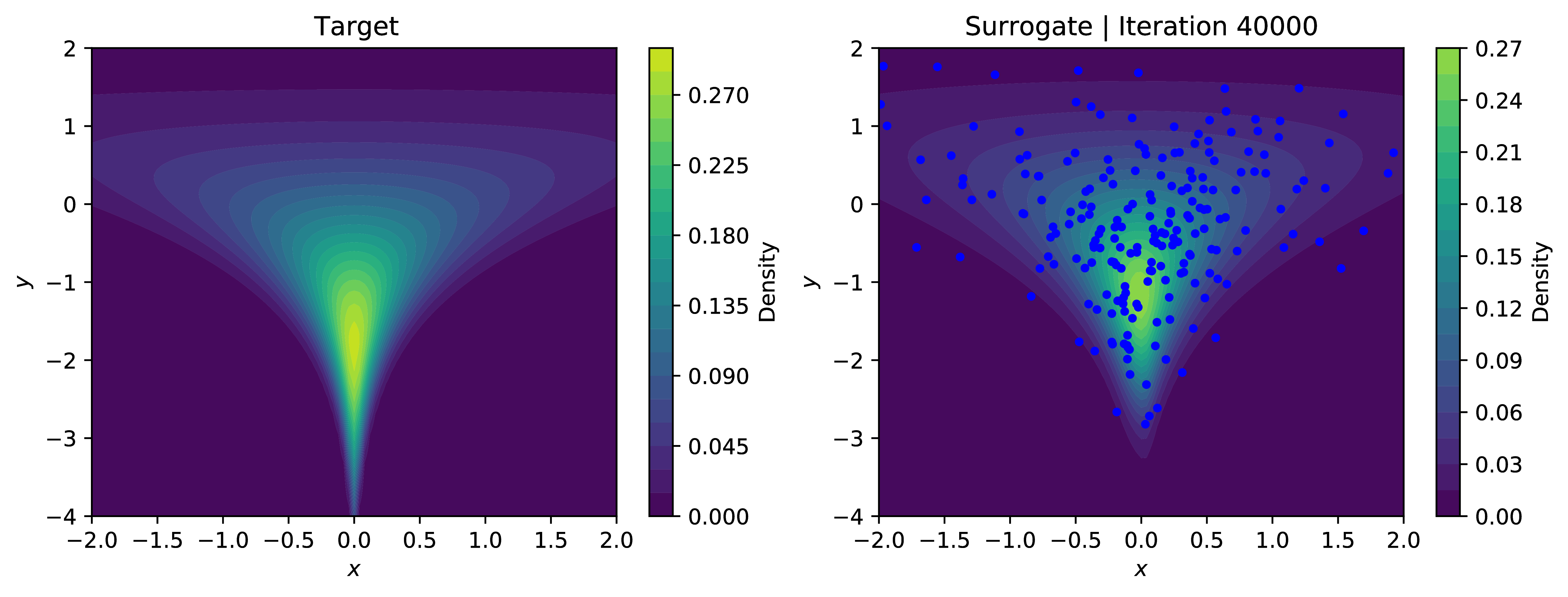
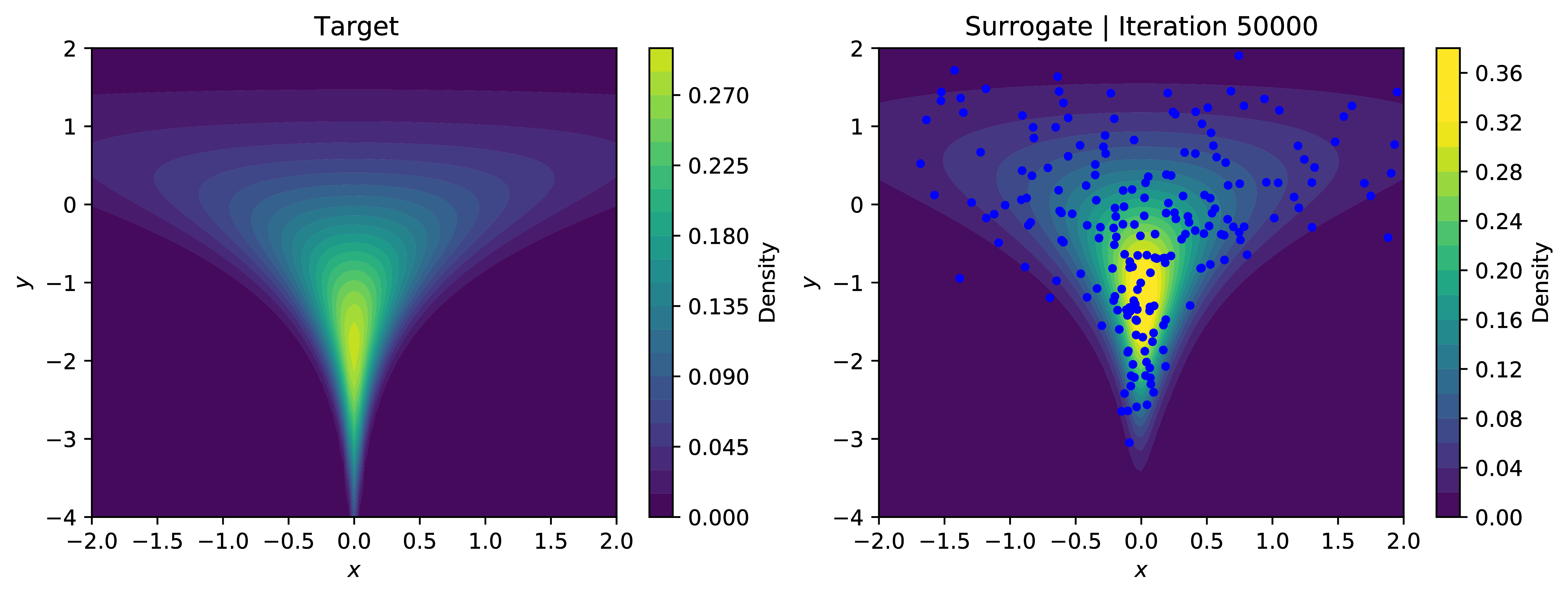
Note the presence of an entropy maximization term in the reverse-KL objective - this translates to minimization of $\log p_{\theta}(x)$ for samples drawn from the surrogate $p_{\theta}$. If we only have access to a lower bound of $\log p_{\theta}$, as in the case of the standard ELBO, then we are minimizing a lower bound - of course, this is in the morally wrong direction. A decrease in the objective can be achieved by deterioration of the tightness of the bound - i.e. an increase in bias rather than actual minimization of $\log p_{\theta}(x)$. The target distribution $p^*$ in this case is defined as (originally proposed by Neal, 2003 [4]):

import jax.scipy.stats.norm as norm
def funnel_log_density(x):
    return norm.logpdf(x[0], 0, jnp.exp(x[1])) + \
           norm.logpdf(x[1], 0, 1.35)

The distribution is shaped like a funnel (see Section 3.3.), with a sharp neck in $x_0$ as the variance is exponential in $x_1$. Note we can straightforwardly sample from $p^*$ by reparameterization: $x_0 = \exp(x_1) \cdot \epsilon$, $x_1 = 1.35 \cdot \epsilon$, where $\epsilon \sim \mathcal{N}(0,1)$, but we’ll see how SUMO fares.

3.1. Objective Function

First we’ll define a function that allows us to sample from the surrogate model. Here we sample from the latent prior and then pass this through the amortized decoder to yield samples $x \sim p_{\theta}$.

def generate_samples(rng, enc_params, dec_params, x=None):
    x_rng, z_rng = random.split(rng, 2)

    if x is None:
        # Sample from standard Gaussian prior
        mu_z, logvar_z = jnp.zeros(latent_dim), jnp.zeros(latent_dim)
    else:
        mu_z, logvar_z = encoder_forward(enc_params, x)
    z_sample = diag_gaussian_sample(z_rng, mu_z, logvar_z)
    mu_x, logvar_x = decoder_forward(dec_params, z_sample)
    x_sample = diag_gaussian_sample(x_rng, mu_x, logvar_x)
    return x_sample

Next we specify a function, reverse_kl, that evaluates the reverse-KL objective for a single example between the target log_prob and our model estimate log_px_estimator. The function batch_reverse_kl applies the vectorizing operator to the single-sample reverse_kl function so we can operate over a batch of samples. Again, the objective functions are made functionally pure by requiring the model parameters as arguments.

def reverse_kl(log_prob, log_px_estimator, rng, enc_params, dec_params):
    """
    Single-sample Monte Carlo estimate of reverse-KL, used to 
    approximate the target density p*(x)

    D_KL(p(x) || p*(x)) = E_p[log p(x) - log p*(x)]
    """
    z_sample, x_sample, qzCx_stats, pxCz_stats = generate_samples(rng, enc_params, 
        dec_params, x=None)
    log_px = log_px_estimator(x_sample, rng, enc_params, dec_params, K, m)
    reverse_kl = log_px - log_prob(x_sample)

    return log_px, reverse_kl

def batch_reverse_kl(log_prob, log_px_estimator, reverse_kl, rng, enc_params, 
                     dec_params, num_samples):
    # Average over a batch of random samples.
    rngs = random.split(rng, int(num_samples))
    vectorized_rkl = vmap(partial(reverse_kl, log_prob, log_px_estimator), 
        in_axes=(0, None, None))
    log_px_batch, reverse_kl_batch = vectorized_rkl(rngs, enc_params, dec_params)
    return jnp.mean(reverse_kl_batch)

3.2. Optimization

Jax natively provides a suite of optimizers for use. In order for the optimization procedure to be functionally pure, optimizers in Jax are defined as an (init_fun, update_fun, get_params) triple of functions:

• init_fun sets the initial optimizer state from the initial values of the model parameters:

opt_state = opt_init(init_model_params)

• update_fun updates the internal state of the optimizer, based on the gradients of the objective function with respect to the model parameters:

opt_state = update_fun(t, gradient, opt_state)  # t: iteration index

• get_params returns the updated model parameters extracted from the internal optimizer state.

model_params = get_params(opt_state)

The end result is that the model parameters are passed into their respective optimizers, and the updated model parameters are returned after taking some gradient step. We’ll use the ubiquitious Adam optimizer, defining separate optimizers for the amortized encoder and decoder.

dec_opt_init, dec_opt_update, get_dec_params = optimizers.adam(step_size=5e-5)
dec_opt_state = dec_opt_init(init_decoder_params)

enc_opt_init, enc_opt_update, get_enc_params = optimizers.adam(step_size=5e-5)
enc_opt_state = enc_opt_init(init_encoder_params)

Armed with this knowledge, we can package together gradient calculation and parameter updates for the encoder and decoder into separate functions. Note below the parameters of the encoder are optimized to minimize the variance of the SUMO estimator.

@partial(jit, static_argnums=(3))
def objective(t, enc_params, dec_params, maximize=False, num_samples=64):
    rng = random.PRNGKey(t)
    reverse_kl_batch = batch_reverse_kl(funnel_log_density, SUMO, reverse_kl, rng, 
                                        enc_params, dec_params, num_samples)
    if maximize is True:
        return jnp.negative(reverse_kl_batch)
    return reverse_kl_batch

@jit
def dec_update(t, dec_opt_state, enc_opt_state):
    # Minimize objective w.r.t. decoder parameters
    enc_params = get_enc_params(enc_opt_state)
    dec_params = get_dec_params(dec_opt_state)
    gradient = jax.grad(objective, argnums=2)(t, enc_params, dec_params, False)
    dec_opt_state = dec_opt_update(t, gradient, dec_opt_state)

    return get_dec_params(dec_opt_state), dec_opt_state

@jit
def enc_update_sumo(t, dec_opt_state, enc_opt_state, num_samples=128):
    # Minimize variance of SUMO w.r.t. encoder parameters
    rng = random.PRNGKey(t)
    rngs = random.split(rng, int(num_samples))
    enc_params = get_enc_params(enc_opt_state)
    dec_params = get_dec_params(dec_opt_state)
    
    def _sumo_sq(rngs, enc_params, dec_params):
        vectorized_rkl = vmap(partial(reverse_kl, funnel_log_density, SUMO), 
            in_axes=(0,None, None))
        log_px_batch, _ = vectorized_rkl(rngs, enc_params, dec_params)
        return jnp.mean(jnp.square(log_px_batch))
        
    enc_gradient = jax.grad(_sumo_sq, argnums=1)(rngs, enc_params, dec_params)
    enc_opt_state = enc_opt_update(t, enc_gradient, enc_opt_state)

    return get_enc_params(enc_opt_state), enc_opt_state 

Note when taking gradients the argnums argument to jax.grad indicates the argument that the gradient of the function should be computed with respect to. Finally, we write a succinct training loop⁴. A callback function is included to plot the learned densities periodically:

total_iterations = 1e5
for t in range(int(total_iterations)):

    # Sample concrete value of K
    K = jit(sampling_tail)(random.PRNGKey(t))
    dec_params, dec_opt_state = dec_update(t, dec_opt_state, enc_opt_state)
    enc_params, enc_opt_state = enc_update_sumo(t, dec_opt_state, enc_opt_state)

    if t % 5000 == 0:
        callback(t, params=(enc_params, dec_params))

If you are interested in the full codebase, you may find it in the repository associated with this post.

3.3. Contour Density Plots

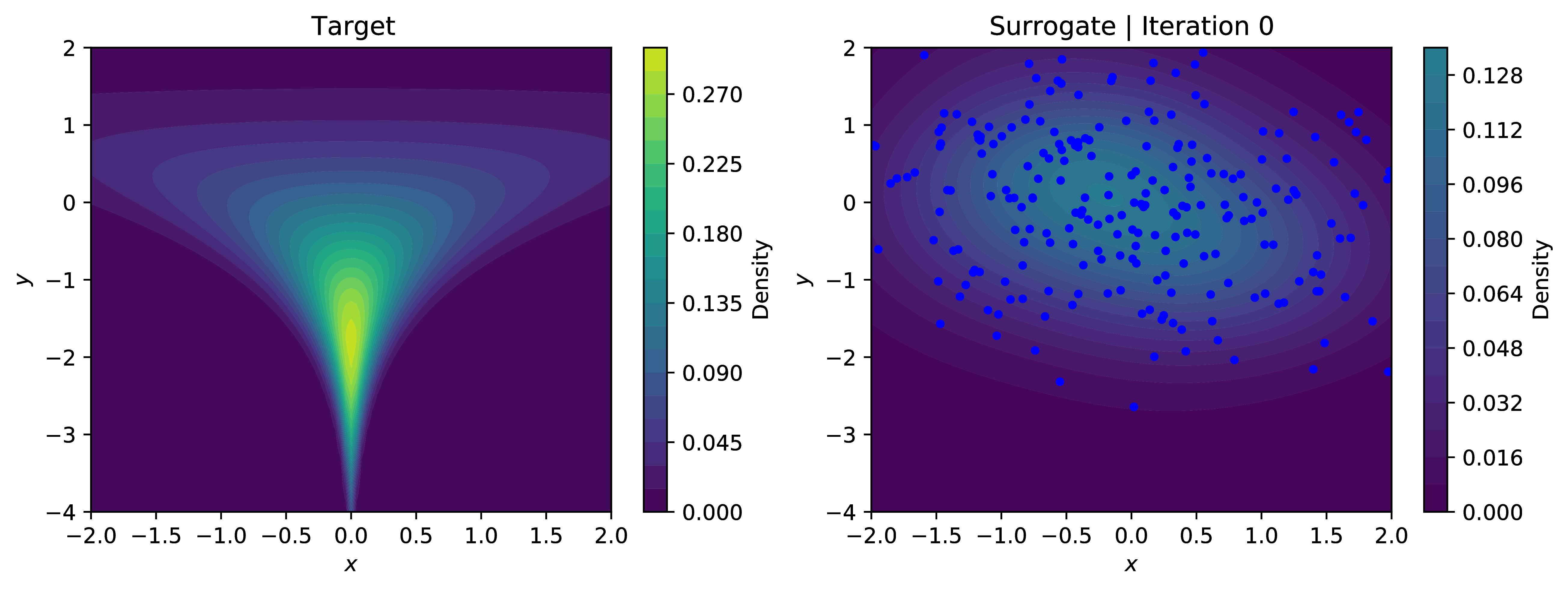
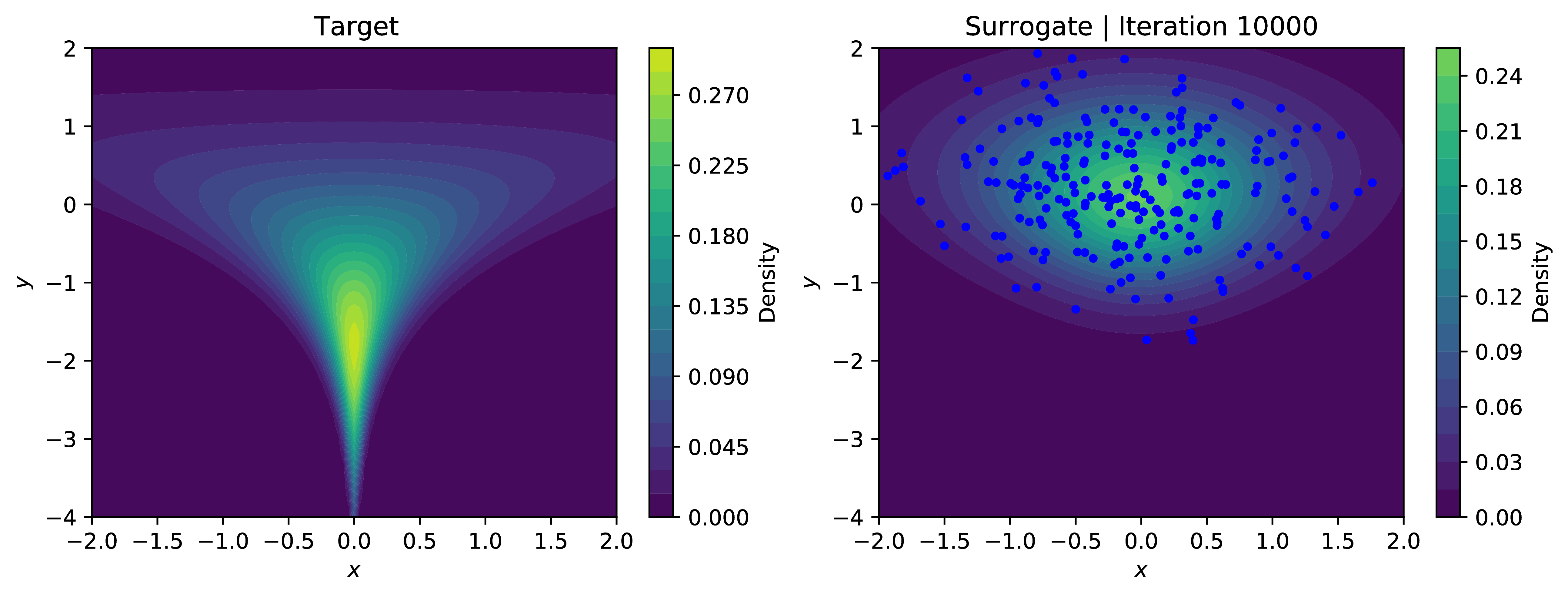
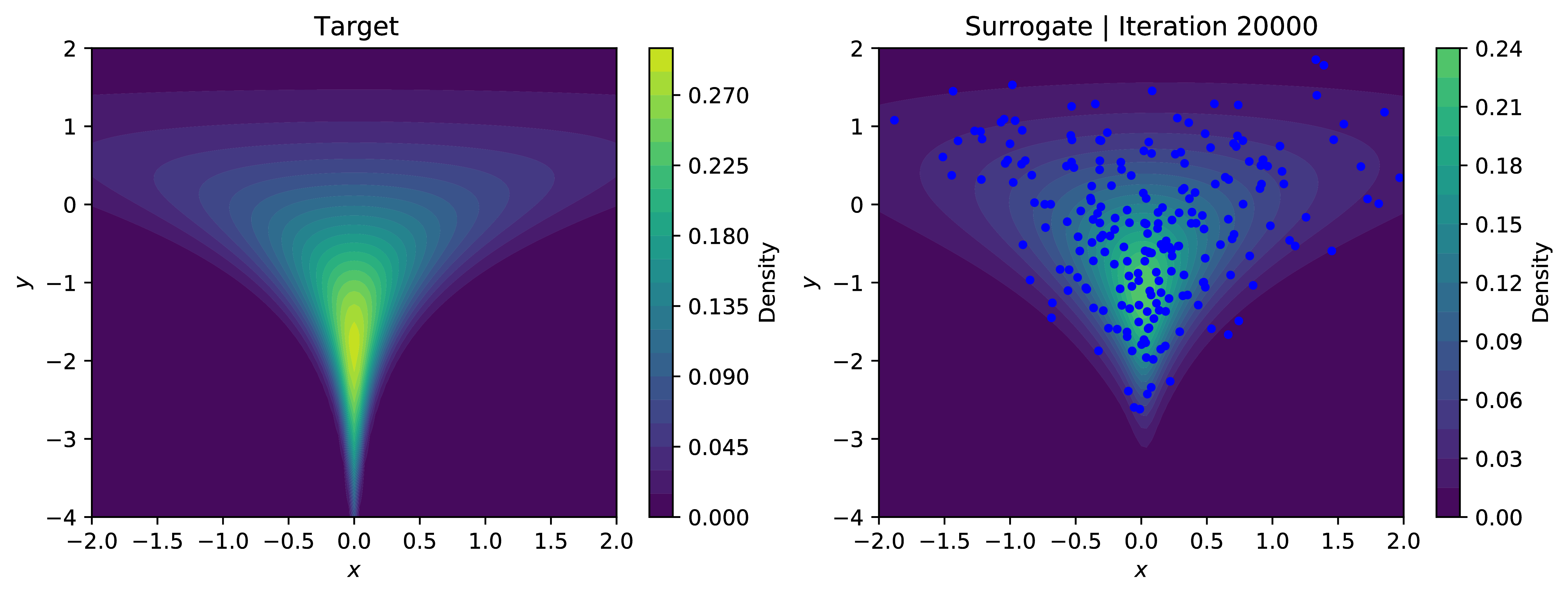
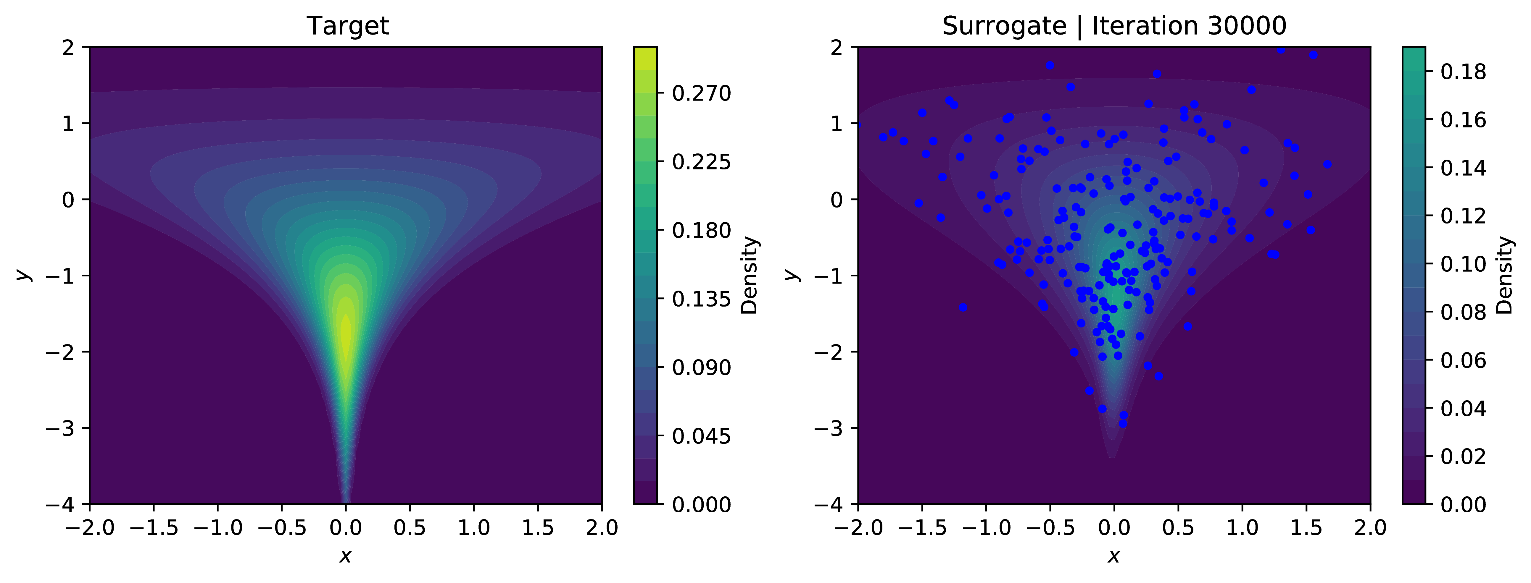
Approximating the log-evidence of our surrogate model using SUMO and minimizing the reverse-KL objective allows our modest approximate sampler to learn the contours of the density; even handling the problematic neck of the funnel relatively well, excepting very low values in $y$. The below plots show the contours of the learned density with samples overlaid in blue. Training using SUMO is significantly more stable than using the IWELBO estimator for similar expected values of compute - for low values ok $K$, the KL-objective optimized under the IWELBO model eventually turns negative and veers toward instability, indicating the model is optimizing the bias rather than the actual objective.

This was just a toy application for an unbiased estimator of $\log p_{\theta}(x)$. In the paper [1], they apply this to more useful problems such as classic density estimation and entropy regularization in reinforcement learning.

Conclusion

Jax has some very interesting design choices. In particular, automatic vectorization through vmap helps with mental overhead a lot once you don’t have to carry around a cumbersome batch dimension. Personally, there’s not enough of a QoL improvement at the moment over Torch for me to port my existing libraries to Jax, but I do enjoy tinkering with it and its minimalism lends itself well to quick proof of concept sketches (provided you are well-acquainted with the sharp edges). One nice use I found for it is a quick way to check correctness of Jacobian determinants computed by hand. Next in this unofficial series we might implement some interesting, possibly continuous, normalizing flow variants, which could be really easy, or troublesome, depending on the behaviour of jax.jit.

Credits

1. Rob Lange’s blog post was very helpful when wrangling over the optimization process for Jax.
2. The (quite large) Jax FAQ helped out a lot when I was banging my head against my keyboard - Jax error traces can be cryptic at the best of times. Hopefully this is one of the rough edges to be ironed out as development continues.
3. Cory Wong for providing the soundtrack for this post.

References

[1] Luo, Yucen, et. al. SUMO: Unbiased Estimation of Log Marginal Probability for Latent Variable Models. International Conference on Learning Representations (2020). https://openreview.net/forum?id=SylkYeHtwr

[2] Burda, Yuri and Grosse, Roger and Salakhutdinov, Ruslan. Importance Weighted Autoencoders. International Conference on Learning Representations (2016).

[3] Lyne, Anne-Marie, et.al. On Russian Roulette Estimates for Bayesian Inference with Doubly-Intractable Likelihoods Statistical Science. Institute of Mathematical Statistics, (2015).

[4] Neal, Radford M. Slice Sampling. Annals of Statistics 31 (3): 705–67 (2003).

You made it!